Click here to see my recommended reading list.
What is Independent Component Analysis (ICA)?
If you’re already familiar with ICA, feel free to skip below to how we implement it in Python.
ICA is a type of dimensionality reduction algorithm that transforms a set of variables to a new set of components; it does so such that that the statistical independence between the new components is maximized. This is similar to Principle Component Analysis (PCA), which maps a collection of variables to statistically uncorrelated components, except that ICA goes a step further by maximizing statistical independence rather than just developing components that are uncorrelated.
Like other dimensionality reduction methods, ICA seeks to reduce the number of variables in a set of data, while retaining key information. In the example we lay out in this post, the variables represent pixels in an image. One of the motivations behind using ICA on images is to perform image compression i.e. rather than storing thousands or even millions of pixels in a image, the storage of the independent components takes up much less memory. Also, by its nature, ICA extracts the independent components of images — which means that it will find the curves and edges within an image. For example, in facial recognition, ICA will identify the eyes, the nose, the mouth etc. as independent components.
ICA can be implemented in several open source languages, including Python, R, and Scala. This post will show you how to do ICA in Python with scikit-learn.
For more information on the mathematics behind ICA and how it functions as an algorithm, see here. Also, for a contrast between ICA and PCA, check out this Udacity video.
ICA with Python
First, let’s load the packages we’ll need. The main functionality we want is the FastICA method available from sklearn.decomposition. We’ll also load the skimage package, which we’ll use to read in a sample image, and pylab which will show the image to the screen (you may need this if you’re using an IPython Notebook).
# load packages
from sklearn.decomposition import FastICA
from pylab import *
from skimage import data, io, color
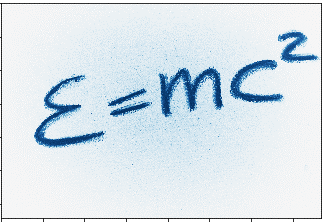
Next, we read in the image. We will set the parameter, as_grey, equal to True. This will make every pixel in the image a value between 0 and 255, rather than a 3-dimensional RGB value. For more information, see this link.
emc2_image = io.imread("emc2.png", as_grey = True)

Now, we choose a number of components we want, and use that number to create a FastICA object. In the sample below, we’ll create a FastICA object with 10 components. This will allow us to run ICA on our image, resulting in 10 independent components.
ica = FastICA(n_components = 10)
Then, we use our object, ica, to run the ICA algorithm on the image.
# run ICA on image
ica.fit(emc2_image)
An important test when doing any type of dimensionality reduction to test how much information has been lost. In our example, we will reconstruct the image with the independent components — i.e. how does the image look if we only know the 10 independent components we’ve developed?
# reconstruct image with independent components
emc2_image_ica = ica.fit_transform(emc2_image)
emc2_restored = ica.inverse_transform(emc2_image_ica)

# show image to screen
io.imshow(emc2_restored)
show()

As you can see, using just 10 independent components still shows a very recognizable version of our original picture. What happens if we change the number of components?
One Component

Three Components

Five Components

Ten Components
Twenty Components

By five independent components, our image is fairly recognizable. After twenty components, our image looks very similar to the original version.
ICA has many other applications, including analyzing stock market prices, facial recognition, and more.